Using Excel for SEO – 16 Tips to Enhance Your Productivity

Adam Brown 6 years ago

As an SEO, data is at the core of everything you do - at least it should be! Dealing with large amounts of data can be a very daunting endeavour. However, Excel is a great tool to automate a lot of the data filtering and formatting tasks, which would take hours to do manually, especially when dealing with large data sets.

Throughout this post we will be giving you a list of 16 Excel formulas and tips you can use to increase your productivity when dealing with large amounts of data.

You can download our Excel for SEO cheat sheet to see working examples of the formulas to keep to hand and use in future by clicking the button below:

So here we go, follow me through this piece to gain a good overview of the formulae you'll need.

Make text / URLs all in lowercase (=LOWER)

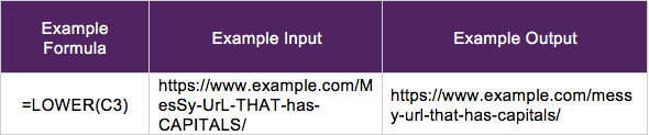
Using this formula makes the highlighted cell into lower case values. This is useful for redirects when a client has uppercase characters within URLs to make them as clean as possible for search engines.

Make text all in capitals (=UPPER)

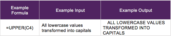
This formula transforms the cell data into all uppercase characters, which is not really needed within the SEO world as you would just use CSS to transform the text, rather than using capitals manually. However, it’s an option to make certain data stand out such as months of the year, or headings within the Excel spreadsheet.

Capitalise beginning of every word (=PROPER)

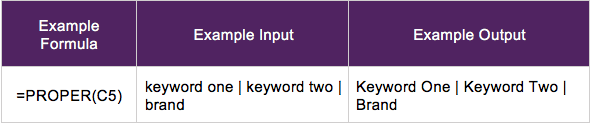
This formula is very useful for quickly formatting title tags. It transforms the start of each word capitalised so they appear more prominent within search engines - which is useful as keyword planner exports tend to be all lowercase values.

Display the character length of a cell (=LEN)

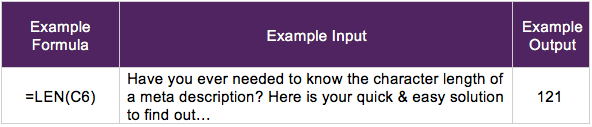
This formula is useful to determine the character length of meta description and title tags. Obviously Google now uses pixel width to display these elements, but it’s a great way to quickly see if you are close to being cut off in SERPs without checking the pixel length.

Count how many times "X" is mentioned within the selected range (=COUNTIF)

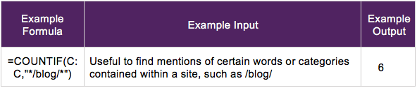
This formula is useful to see how many times a value is mentioned within the document. This can be used to see how many pages are equated to the top level folder structure easily, such as /blog or /product-category/.

Or this formula can be used to identify any duplication, cannibalisation or over-optimisation across the website content/title tags, etc. This will give you the number of times it is mentioned across the selected range.

Give more of a description of an error (=IFERROR)

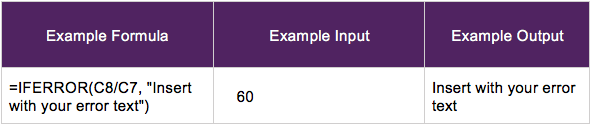
This formula helps to give the user a bit more guidance on any errors being shown that the default Excel displays such as: #N/A, #VALUE!, #REF!, #DIV/0!, #NUM!, #NAME?, or #NULL!. This can be useful if your client developers have access to any of your files, and to guide them if they have made any errors.

Merge multiple column of data into one cell (=CONCATENATE)

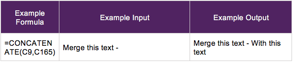
This formula is great to merge a lot of data together, such as keywords & locations, root domains & sub folders. Then copy and paste the column as text only and it remains static within the Excel sheet; super useful when dealing with a lot of variable elements.

Find the average of the data range selected (=AVERAGE)

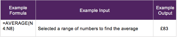
This is a simple formula to find the average of a selected data range. This can be very useful for the average keyword rank. However, this comes with some pitfalls.
For example, if a keyword only had 10 search volume, but dropped out of the top 500 of Google, this would have a drastic effect on the average rank. Later on, we'll look at how to do a weighted average keyword based on search volume to give a better representation of keyword growth for your clients.

Extract data from the left, middle or right of a cell (=LEFT / =MID / =RIGHT)

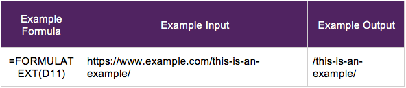
This formula is great to quickly extract a certain element from a URL or text into a different cell. It could be useful to a multitude of applications such as extracting the root domain, top level folders, WWW’s, HTTP or cutting off text after the set limit.

Find & replace without the Internal Excel function (=SUBSTITUTE)

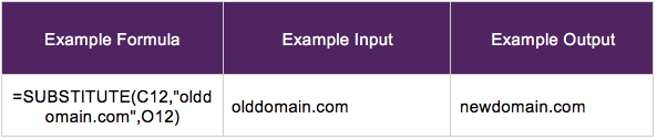
This formula basically acts as the find & replace function within Excel. However, you can be a lot more concise with this method as you can see the change side by side, instead of replacing it completely, then reverting back if it wasn’t what you expected.

Remove blank spaces within cells (=TRIM)

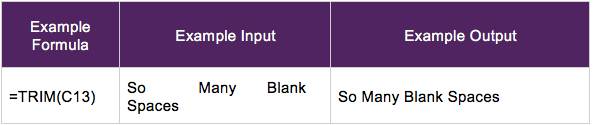
Do you ever copy text from somewhere with weird formatting, or multiple blank spaces within the cell? If so, you can quickly remove all of the blank spaces within the selected cells by implementing this formula.

Comparing data from two different tables (=VLOOKUP / =HLOOKUP)

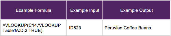
VLOOKUPs & HLOOKUPs are very useful ways of pulling out unordered data from different tables or sheets contained within the Excel document.

Use VLOOKUP when values are situated in the first column of a table with information organised vertically. Use HLOOKUP when lookup values are situated in the first row of a table. An example of when to use this is when you export a product list of ID numbers, then need to pull off the product's name, price or weight.

Convert URLs into text links (=HYPERLINK)

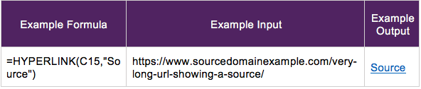
This formula comes in handy if you’re doing a lot of competitor/keyword research and need to cite the sources within Excel. Instead of having inconsistent column sizes, you can create a simple 'source' hyperlinks. To do the opposite & extract URLs from text links, you can setup a macro which is explained here, which is also very handy.

If cell contains word mark as “X” (=IF)

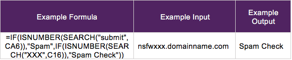
This formula is useful for link and content audits as you can mark specific known spam keywords, to show which areas you need to review first.

Weighted average keyword rank based off search volume (=SUMPRODUCT)

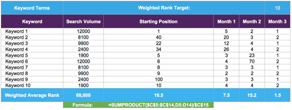
Download the resource for this graph.

This formula is very good for showing the performance of keywords taking into account their search volumes and current positions. The problem with the traditional average formula is that if a low search volume keyword dropped 20 positions, but a high search volume keyword gained five positions, the average position would reflect negatively, but in theory you would be gaining more organic traffic from the result of this.

This formula solves this issue by adding the search volume and current positions together, then dividing the total value against search volume to display the weighted average rank score. Placing a dollar sign in a formula tells Excel that you don’t want it to adjust the range reference when you copy the formula to the other cells.

Pivot Tables

Pivot tables are a useful tool for displaying key points from a large pool of data.
They can be easily moved around and help the user by providing expandable and collapsing sections, allowing both a detailed and overarching view of the filtered data.

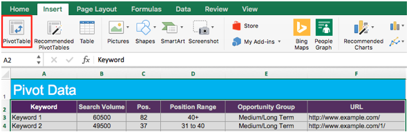
A working example we have created within the downloadable document is when you have a large set of keyword data along with the positions, search volume and URLs.

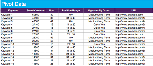
As you can see, it would take a while for a client to decipher what this data means and to highlight any sort of actionable points. To paint a clearer picture for this data, if you highlight the selected cells, then select 'insert' on the tab at the top and click pivot table.

You will then be presented with the pivot table builder on the right, where you need to specify the rows, columns, values and filters if needed. If you use the following format below, you will get a table like the following on the left:

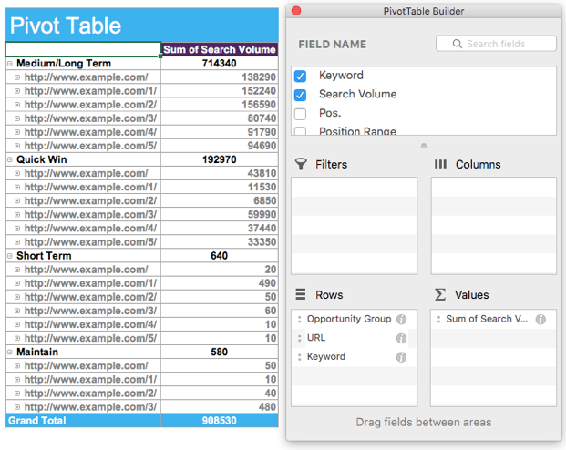
As you can see, using this format clearly shows the search volume - by opportunity group, then by URL - and the user can dive further into the data by seeing which keywords are behind this data. For example:

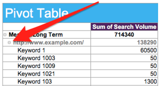
This allows the user to see which areas they should be focusing on based on search volume, current positions within search engines and what URLs have the most opportunity for growth - all within minutes of creating a filtered pivot table.

Overview

I hope you have learned something new from this guide that will help you become more proficient using Excel for SEO activity. Be sure to download the cheat sheet to keep a record of these all important formulas and tables mentioned throughout this post.

Are there any Excel formulas that you can’t live without? Share your thoughts below in the comments.